Pandas Groupby and Pivot Tables

Introduction

This is the third article in a series on pandas, the ubiquitous data analysis and manipulation software library written in Python. If you are new to the pandas module then you're encouraged to take a look at the earlier articles in this series before continuing with this one.

• Part 1 is an introduction to pandas and covers setup, the DataFrame object, importing raw data, slicing, selecting, and extracting values from a DataFrame. 
• Part 2 covers boolean indexing and DataFrame sorting.

In this tutorial we are going to cover the pandas groupby function, take a look at DataFrame stacking, and learn how to build pivot tables (pandas.pivot_table) from our raw data.

Sample Dataset

We will make use of the same classic car dataset that we've used in the first two pandas tutorials to illustrate grouping and pivot tables. The dataset was originally sourced from Kaggle and is available to download here if you wish to follow along.

Once pandas has been installed, import the package into a new script or notebook and read the raw data into a new DataFrame.

import pandas as pd

filename = 'classic-cars.csv'
df = pd.read_csv(filename,index_col='car')

The DataFrame is indexed using the 'Car' column and consists of 406 rows representing different classic cars, and 8 column attributes describing each vehicle.

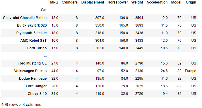
With the DataFrame loaded we are ready to move on to DataFrame grouping.

Pandas Groupby Function

The groupby function is called on an existing DataFrame, and allows you to modify the presentation of the dataset by grouping data either by a column or a series of columns. 

A typical groupby operation will consist of one or more of the following steps:

• A split of the data into groups based on some criteria.
• The application of a function to those split groups.
• A combining of the results into a data structure (typically a new DataFrame) .

Let's take a closer look at the groupby function.

DataFrame.groupby(by=None, axis=0, level=None, as_index=True, 
                  sort=True, group_keys=True, squeeze=NoDefault.no_default, 
                  observed=False, dropna=True)

• by is one or more columns in the DataFrame around which you will group the data. We'll cover grouping both by one column and multiple columns in the examples that follow. A function can also be passed to by which will be called on each value of the object's index. The columns passed to by will form the rows of the newly grouped DataFrame.
• axis determines whiether to split along rows (0) or columns (1).
• level is used to group by a particular level or levels in a MultiIndex DataFrame. We'll cover MultiIndexing later in the tutorial.
• Refer to the groupby API for more detailed information on the function parameters.

Aggregating the Group

The application of the groupby method is one of two steps commonly performed when grouping data into a new DataFrame. The second step involves aggregating the split data to produce some additional insight from the dataset. The aggregation function is called directly after the groupby and is usually one of the following operations: 

• .sum() to sum the grouped data
• .mean() to average the grouped data
• .min() or .max()
• .size() to find the number of entries in the group (including NA values)
• .count() to count the entries (excluding NA values)

This two step grouping and aggregating process is best shown through a set of examples. Let's dive straight in and perform some grouping using our classic car dataset.

Group By a Single Column

The "Origin" column in our classic cars dataset gives an indication where in the world each car was designed and manufactured. It would therefore be useful to group the cars by region, to then look for similarities and differences between the resulting groups.

Since we have a differing number of cars from each region our first aggregation function should be a mean() to provide us with the average column attributes of the vehicles per region.  

cars_by_origin = df.groupby('Origin').mean()
cars_by_origin.sort_values('MPG')

The first line in the codeblock above groups our dataframe by "Origin" and then applies a mean to the grouped data. The second line simply sorts the resulting DataFrame by fuel efficiency ("MPG") from least efficient to most efficient. 

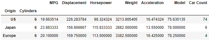
The output is a DataFrame, displayed below.

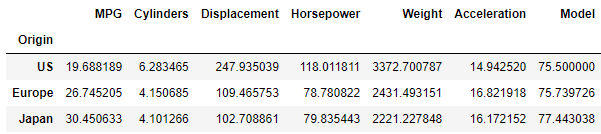
The rows of the DataFrame are now grouped by origin and the columns are the mean values of the remaining column attributes. This aggregated view of our original data provides some new insights:

1. US cars are generally far less fuel efficient than their European and Japanese counterparts.
2.  US cars are on average heavier, and their engines are larger (displacement), more powerful (horsepower) and on average contain two additional cylinders relative to the cars from Europe and Japan. This provides an initial explanation for the relatively poor fuel consumption of the US cars — the cars are simply larger and more powerful.

Group by Multiple Columns

The grouping of car data by region is interesting and immediately highlights some clear divergence in car design methodology across the regions. It would be interesting to take the analysis a step further and see whether the differences identified by averaging all cars per region still exist when comparing cars per region with similar sized engines.

To do this we need to add a second criterion to groupby. Now we will first group by "Origin" and then perform a second grouping by the number of cylinders that each engine has. This will allow us to compare like-for-like cars with similar engines between the different regions.

We'd also like to total the number of cars in each sub-group (region and number of cylinders) to get an idea of the relative sizes of the datasets. The code to perform this is shown in the block below.

# DataFrame groupby of multiple columns
car_grouping = df.groupby(by=['Origin','Cylinders'])
car_numbers = car_grouping.size()
car_types_by_origin = car_grouping.mean()
car_types_by_origin['Car Count'] = car_numbers

• Pass a list of column names to the by parameter. Grouping will occur in the order the names appear in the list.
• The size() method peforms a count of the number of cars in each group.
• The average values in each group are calculated when aggregating by mean().
• A column named "Car Count" is added to the grouped and aggregated dataframe showing the total number of cars in each sub-group.

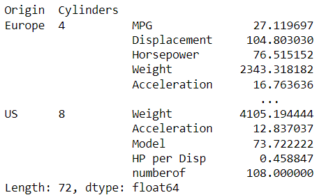
The resulting DataFrame is shown below.

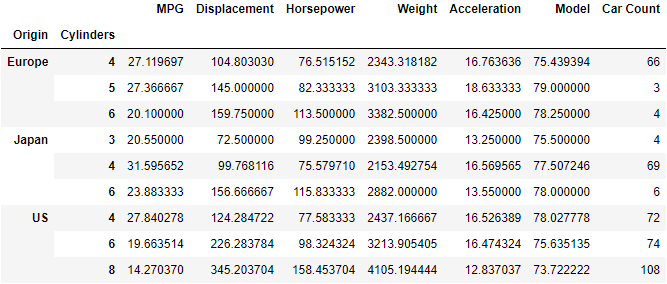
Our DataFrame is now defined by two indexes, "Origin" and "Cylinders". Calling car_types_by_origin.index results in a MultiIndex object. The two indexes corresponding to a row in the DataFrame are now housed in a tuple.

>>> print(car_types_by_origin.index)
"""
MultiIndex([('Europe', 4),
            ('Europe', 5),
            ('Europe', 6),
            ( 'Japan', 3),
            ( 'Japan', 4),
            ( 'Japan', 6),
            (    'US', 4),
            (    'US', 6),
            (    'US', 8)],
           names=['Origin', 'Cylinders'])
"""

The MultiIndex DataFrame is a convenient way to perform a more like-for-like comparison between the vehicles manufactured in the different regions as we've now additionally split the vehicles in each region by the size of the engine (approximated here by the number of cylinders).

Let's now examine how to extract specific information from the MultiIndex Dataframe.

Extract a Row from a MultiIndex DataFrame

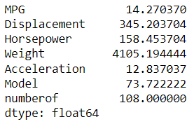
We can extract a row from the DataFrame (will be output as a series) by making use of the naming conventions given by the index method we wrote out above. Rows are named by a tuple corresponding to the grouping of the data. The loc method is used to extract rows from the DataFrame and so the MultiIndex row is output as follows:

# extract the information on US model cars with 8 cylinders
>>> print(car_types_by_origin.loc[("US",8)])
"""
MPG               14.270370
Displacement     345.203704
Horsepower       158.453704
Weight          4105.194444
Acceleration      12.837037
Model             73.722222
Car Count        108.000000
Name: 8, dtype: float64
"""

To extract a specific attribute from the grouped data (one entry) then just call that attribute after the loc function that outputs the series.

# average Horse power of US 8 cylinder cylinder cars
>>> print(car_types_by_origin.loc[("US",8)]['Horsepower'])
158.4537037037037

Extract Multiple Rows from a MultiIndex DataFrame

Taking a further look at the car_types_by_origin DataFrame that we have created it may be easiest to compare cars like-for-like by showing only the cars with equal numbers of cylinders from each region. This would make for an easier comparison.

This is easy to do as we know how to extract a single row using the index tuple. Multiple rows are extracted by creating a list of tuples corresponding to the rows we wish to extract.

# create a DataFrame of cars from each region with 4 cylinders
four_cyl_compare = car_types_by_origin.loc[[("US",4),("Japan",4),("Europe",4)]]

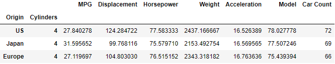
Previously we had noted fairly large differences in the average engine size and fuel consumption between cars manufactured in the US relative to those from Europe and Japan. However, when we examine similar cars (4 cylinder engines) we see that the equivalent small US cars are actually very comparable across all dimensions.

To complete this section let's also show the comparison between six cylinder cars.

six_cyl_compare = car_types_by_origin.loc[[("US",6),("Japan",6),("Europe",6)]]

This actually ends up being quite interesting as on average US six-cylinder cars have bigger engines (larger displacement) but are down on power (Horsepower) relative to the others. The European and Japanese engines are more efficient in how they generate power (more power for smaller displacement) and consequently show improved fuel consumption relative to the US engines.

Stack and Unstack DataFrames

There are some instances when you need to reshape a DataFrame to better suit the analysis you are performing. Two common methods are the stack and unstack functions which you can use to restructure columns and rows (index).

DataFrame Stack

A good analogy to DataFrame stacking is to take a row of books that are horizontally orientated and vertically stack them one on top of the other. Stacking in pandas will reshape the DataFrame, and so if a DataFrame with a single level of columns is stacked, the result will be a Series rather than a DataFrame. 

Let's illustrate this with the car_types_by_origin DataFrame previously created. 

stack_cars = car_types_by_origin.stack()

The stacked data stack_cars is a nested Series. The values in the stack are accessed by referring to the index tuple.

We can show that the result of applying the stack() to the DataFrame is to turn that DataFrame into a Series.

print(f"The stacked result is a {type(stack_cars)}.")
"The stacked result is a <class 'pandas.core.series.Series'>."

We can access the inner level of the series using the index tuple. For example, we can show the series in the stack of US 8 cylinder cars as follows:

US_8cylinder = stack_cars[('US',8)] # tuple index to call series

The result is also a series:

Unstack

The inverse of stack is unstack. Applying the unstack method to a stacked series will result in the original DataFrame being displayed.

# unstack is the inverse operation of stack
unstack_cars = stack_cars.unstack()

Pivot Tables

Pandas provides spreadsheet-like pivot table functionality through the pivot_table method. The various levels in the pivot table are stored as MultiIndex objects on the index and columns of the resulting DataFrame.

Let's take a closer look at the pivot_table function.

pandas.pivot_table(data, values=None, index=None, columns=None, aggfunc='mean',
                   fill_value=None, margins=False, dropna=True, 
                   margins_name='All', observed=False, sort=True)

• data is the Dataframe from which you will build the pivot table.
• values refer to the column or list of columns to aggregate. 
• aggfunc is the function, list of functions, or dict of functions to aggregate the columns by. If a single function is passed e.g. 'mean' then that function will be applied to all columns in the pivot table. If you want to apply a different function to the various columns then pass a dict where the dict key is the column name and the dict value is the function to apply. If a list of functions is passd, the pivot table will have hierarchical columns whose top level are the function names.
• index is the key(s) to group-by on the pivot table index.
• columns is the key(s) to group-by on the pivot table column.
• fill_value is the value to replace missing values with (in the resulting pivot table after aggregation). The default is None.
• margins is a bool with default False that when True will create an additional row where the values of all rows/columns will be added and the sub-total or grand totals displayed. The default name for this row is 'All' which can be changed with the margins_name parameter. 
• If you do NOT wish to remove all columns whose entries are NaN then set dropna=False.
• Refer to the official API documentation for further information. 

The best way to see a pivot table in action is to go through a worked example. We'll start with a simple single index pivot table and then move onto a slightly more advanced MultiIndex example.

Single Index Pivot Table

Let's use a pivot table to further investigate the engine differences between cars manufactured in the three regions. One measure of engine efficiency is the amount of power that can be generated from a given engine displacement. It is very easy to create additional columns in pandas and calculate a new value for each entry in that column using the existing columns. We'll do that now and create a "HP per Disp" column.

df['HP per Disp'] = df['Horsepower']/df['Displacement'] # new column

The pivot table is created using the pivot_table method and parameters are added to the function call in the ways described above. We are grouping the data around the vehicle "Origin" column and want to output the mean values across the data on the "Horsepower", "Displacement" and "HP per Disp" columns. We can also add an extra row what takes the mean across all the data to better compare our grouped results by setting margins=True and specifying a margins_name.

col_list = ['Horsepower','Displacement','HP per Disp']

pivot1 = pd.pivot_table(data=df,values=col_list,index='Origin',aggfunc='mean',
                        margins=True, margins_name='All Regions')

pivot1[col_list].sort_values(by='HP per Disp',ascending=False)

The resulting DataFrame is output below. By default the DataFrame will show the columns in alphabetical order, but the order can be changed to aid in explanation by passing a list of column names to the DataFrame in square brackets as shown in the last line of the codeblock above.

Finally it is easier to interpret the result if the values are sorted. In this case we'd like to sort the results by "HP per Disp" from largest (most efficient) to smallest (least efficient).

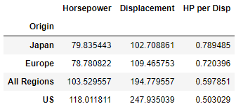
• Japanese car engines on average are the most efficient, generating the most horsepower per cubic inch.
• American car engines are on average much larger than their European and Japanese counterparts — producing the most power but least efficiently.

MultiIndex Pivot Table

One nuance of our dataset not adequately captured in the pivot table created above is that there are a lot of 8 cylinder US cars which may be skewing the results somewhat. There are no Japanese or European 8 cylinder cars in the dataset so it would be useful to perform a more like-for-like comparison and compare the 4 and 6 cylinder cars from each region directly. We can do this be generating a MultiIndex pivot table and then extracting the data we require.

This time we'll index on the "Cylinders" column and split our columns to show "Horsepower", "Displacement" and "HP per Disp" by region. 

agg_values=['Horsepower','Displacement',"HP per Disp"]
pivot2 = pd.pivot_table(data=df,index='Cylinders',values=agg_values,columns='Origin')
pivot2[values]

The resulting pivot table is shown below. NaN values are applied automatically where there is no data available.

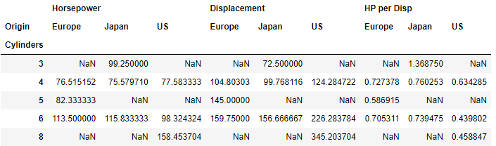
This pivot table DataFrame is still a little difficult to interpet so let's only show the 4 and 6 cylinder rows where data is available for all regions.

Selecting Particular Rows and Columns in Pivot Table

It is easy to filter out the rows and columns we need from the pivot table by applying the loc function to extract rows of interest and using square bracket notation to select the columns. Here we only need to extract "HP per Disp" to compare the efficiency of similar sized engines per region.

pivot2.loc[[4,6]]['HP per Disp']

Now we can directly compare similar engines based on the number of cylinders by region.

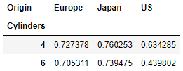
• The US engines are still the least efficient across both common engine sizes.
• The smaller engines (4 cylinder) are more closely matched across all three regions.
• Japanese engines are the most efficient across all common engine sizes.

Wrapping Up

This brings us to the end of this tutorial on pandas grouping and pivot tables. Hopefully by running through some examples using an actual dataset you now have a feel for the power of grouping and pivot tables.

In this article we have covered:

• The groupby function which splits and aggregates a DataFrame to provide new insight into the raw data.
• We discussed stacking and unstacking of DataFrame structures.
• The MultiIndex DataFrame was introduced.
• Pivot tables were built using the pivot_table method which provides powerful spreadsheet like pivot table functionality in just a few lines of code. 

If you missed out on the earlier pandas tutorials you can catch up by checking out the links below:

Introduction to Pandas

Boolean Indexing and Sorting in Pandas

Thanks for reading this pandas tutorial. If you enjoyed it and found it useful then please consider sharing the article using one of the options below.