An Introduction to Pandas

Introduction

If you are using Python to perform any sort of data manipulation and analysis then you are almost certainly going to be doing so using the pandas software library (you would be crazy not to). Pandas states on its website that it "aims to be the fundamental high-level building block for doing practical, real world data analysis in Python" and by all accounts it has achieved exactly that.

In the 2022 Stack Overflow Survey pandas was positioned third in the category of most used other frameworks and libraries (excluding web development) just behind NumPy. 

It is no surprise then that pandas is extensively used alongside NumPy and Matplotlib when working with datasets or performing analysis in Python.

This post is the first in a set of tutorials to introduce the package, and to showcase some of the powerful functionality and features available. Let's dive right in.

Imports

Pandas is a standalone Python package that must be installed before use. Installation can be completed through conda or pip. Many scientific Python distributions are available to download which will all come preinstalled with pandas, and this is the preferred way to quickly get up and running. Working with a scientific Python distribution will ensure that you also have access to NumPy and Matplotlib (among others) which are all essential packages when performing numerical analysis. 

Two commonly used scientific distributions are Anaconda and WinPython, which both come preinstalled with all the packages you need to get started.

The pandas package must to be imported before first use in a script or notebook; the convention is to do so using the abbreviation pd.

We will be working with a real-world dataset throughout this tutorial, and so if you wish to follow along you will also need to import NumPy. 

import numpy as np
import pandas as pd

Data Structures

Before diving in to the actual pandas data analysis and code implementation it is worth spending a little time discussing the two fundamental data structures that pandas is built around. Pandas data is stored in a labelled array object differentiated between a 1D array (series) and a 2D array (DataFrame).

Series (1D)

A series is a one-dimensional labelled array capable of holding any data type (and indeed you can store a mix of data types within the series).

s = pandas.Series(data, index=index)

• data can be any data type but typically a dict or ndarray is used to populate the series.
• The data labels are referred to as the index which is either added as a list or array of the same length as data, or alternatively if data is populated from a dict then the keys of the dictionary are used as the index.

A simple example of creating a series using a dictionary is shown below.

adict = {
    'dog':1.22,
    'cat':3.14,
    'fish':5.66,
}

s = pd.Series(data=adict) # note the capital S

The output is a series object where the dict keys form the index, and the values form the data.

dog     1.22
cat     3.14
fish    5.66
dtype: float64

To access the data in a series you can refer to the index in the same way as you would a dictionary key.

>>> print(s['dog'])
1.22

>>> print(type(s))
<class 'pandas.core.series.Series'>

DataFrame (2D)

a Dataframe is a two-dimensional labelled data structure and is the most commonly used object in pandas. It is helpful to think of a DataFrame as a spreadsheet consisting of rows and columns, or a SQL table.

pandas.DataFrame(data=None, index=None, columns=None, dtype=None, copy=None)

• data refers to the data to be housed in the DataFrame and is most commonly imported from a CSV file or built up from a 2D NumPy array.
• The index is the row labels of the DataFrame.
• The columns are the column labels of the DataFrame. 

By explicitly specifying index and/or columns you are guaranteeing the values to be used for the labelling of the DataFrame. If you do not pass index and column values then pandas will assign values itself. As you will soon see when importing data from a CSV file (a common application) into a DataFrame, the columns and index are easy to set directly.

An example DataFrame is pictured below where the index and columns are labelled.

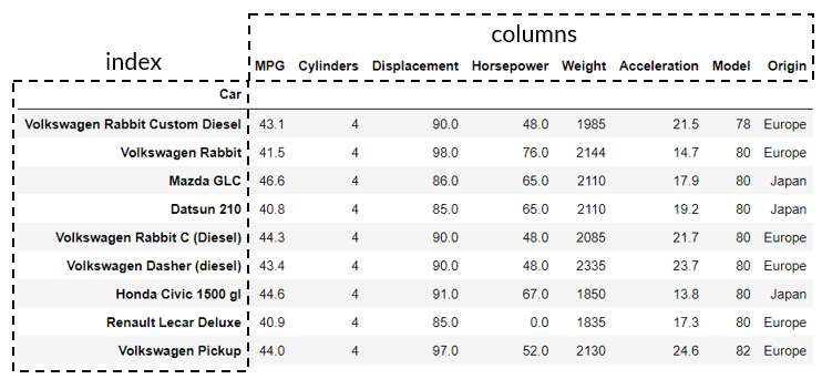
It's best to learn by doing, so let's move onto the specifics of creating a DataFrame and selecting the index and columns next.

Working with DataFrames

Importing from CSV

One of the most common ways to create a DataFrame is through the importing of a set of raw data from a comma-separated values (CSV) file. This is accomplished using the pandas.read_csv method which takes a CSV file as input and returns a pandas DataFrame. Once the raw data is housed in a DataFrame then cleanup, manipulation, and reshaping can all take place using pandas built functionality and methods.

We'll be using an open-source dataset of classic cars for the remainder of this tutorial (and those to follow), which was originally sourced from Kaggle. You can download a copy here if you wish to follow along. 

Start by importing the csv file using the pandas.read_csv method and then take a look at how the file is translated into a DataFrame. 

import pandas as pd

filename = 'classic-cars.csv'
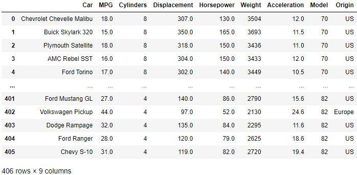
df = pd.read_csv(filename)

The top line of the CSV file has correctly been assigned to the columns, but the rows or index is currently made up of a set of integers from 0 to n where n is the number of rows in the CSV file (minus the first row assigned to the column names).

It is often preferable to index the DataFrame with the data housed in one of the columns as many raw datasets will include an ID or primary key of sorts. To do this you need to add the index_col argument to the read_csv method and select the column in the DataFrame that you wish to use as the index. In this case it makes the most sense to use the 'Car' column as the index.

filename = 'classic-cars.csv'
df = pd.read_csv(filename,index_col='Car')
# the index is set from one of the named columns in the dataframe

The resulting DataFrame is now indexed by the 'Car' column.

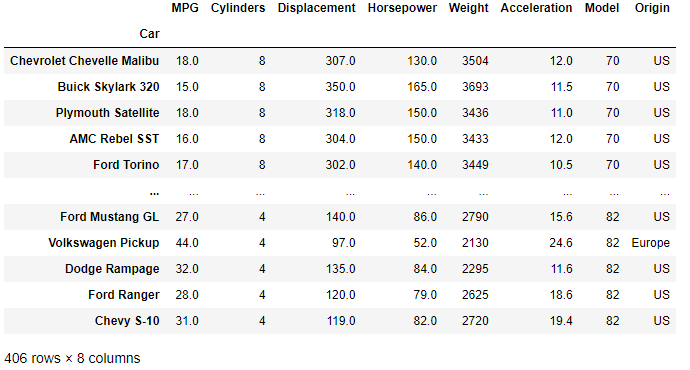
You may notice that the number of columns in the DataFrame has been reduced by 1 when calling 'Car' as the index. This is an important behaviour to be aware of — the index does not form a part of the DataFrame values (i.e. it is not a column of data in the DataFrame) but is still accessible through the index method. We'll discuss this and the shape of the DataFrame next. 

DataFrame Shape

The shape of a DataFrame refers to the number of rows and columns of data in the array object. To extract this information you use the shape method. This returns a tuple of rows,cols.

>>> rows, cols = df.shape
>>> print(f"The dataset has {rows} rows and {cols} columns.")
"The dataset has 406 rows and 8 columns."

Head and Tail

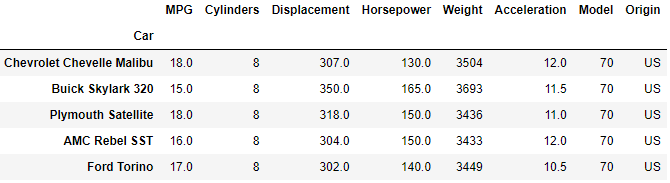
If you want to quickly investigate the DataFrame without loading the entire array (which can be very large and therefore computationally expensive) you can use the head or tail methods which will show you the beginning or end rows of the DataFrame respectively. The default number of rows to display is 5 but this can be changed by providing an argument to the function. This is useful when you first load a DataFrame as it allows you to see how the raw data has been interpreted into the DataFrame format without loading the entire dataset.

df.head()

The tail method shows the last n rows of the DataFrame.

df.tail(3)

Index and Columns

The DataFrame index and columns can be accessed by the index and columns methods respectively. These are of the type Index which is the object that pandas uses to store index and column data. An Index can be easily converted to a NumPy array or a list through the to_numpy and to_list methods respectively.

>>> df = pd.read_csv(path,index_col='Car')

>>> index = df.index
>>> print(type(index))
<class 'pandas.core.indexes.base.Index'>

# convert index to a numpy array
>>> index_array = index.to_numpy()

>>> columns = df.columns
>>> print(columns)
Index(['MPG', 'Cylinders', 'Displacement', 'Horsepower', 'Weight',
       'Acceleration', 'Model', 'Origin'],
      dtype='object')

>>> print(type(columns))
<class 'pandas.core.indexes.base.Index'>

>>> columns_list = df.columns.to_list()
>>> print(columns_list)
['MPG', 'Cylinders', 'Displacement', 'Horsepower', 
 'Weight', 'Acceleration', 'Model', 'Origin']

Selection

Pandas makes it very easy to extract or select data from rows or columns. One important consideration to keep in mind is that when extracting a single row or column from the DataFrame, the resulting data type will be a pandas series object as the resulting row/column is a 1-D array.

Selection by Column

Columns in a DataFrame are selected by referring to the column by its name. You extract a column from the DataFrame in the same way as you would refer to the value in a dict by referencing the dictionary key.

# select of column by name
num_cylinders = df['Cylinders']

Printing out the column will print out a pandas series of length equal to the number of rows in the DataFrame.

>>> print(num_cylinders)
"""
Car
Chevrolet Chevelle Malibu    8
Buick Skylark 320            8
Plymouth Satellite           8
AMC Rebel SST                8
Ford Torino                  8
                            ..
Ford Mustang GL              4
Volkswagen Pickup            4
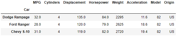
Dodge Rampage                4
Ford Ranger                  4
Chevy S-10                   4
Name: Cylinders, Length: 406, dtype: int64
"""

>>> print(f"The data type is {type(num_cylinders)}.")
"The data type is <class 'pandas.core.series.Series'>."

An alternate way of referencing a column is through dot notation. Here the column name (not a string) is added to the DataFrame variable as you would a method.

# using dot notation
df.Weight
"""
Car
Chevrolet Chevelle Malibu    3504
Buick Skylark 320            3693
Plymouth Satellite           3436
AMC Rebel SST                3433
Ford Torino                  3449
                             ... 
Ford Mustang GL              2790
Volkswagen Pickup            2130
Dodge Rampage                2295
Ford Ranger                  2625
Chevy S-10                   2720
Name: Weight, Length: 406, dtype: int64
"""

Selection by Row

There are two pandas methods that can be used to select a particular row of a DataFrame. The loc method selects by index name and the iloc method by the index number.

Row Selection by loc

A row can be selected by name using the loc method as demonstrated below.

my_car = df.loc['Ford Ranger']
print(my_car)

The result is a pandas series object.

"""
MPG              28.0
Cylinders           4
Displacement    120.0
Horsepower       79.0
Weight           2625
Acceleration     18.6
Model              82
Origin             US
Name: Ford Ranger, dtype: object
"""

Row Selection by iloc

To select a row by the index you use the iloc method. The input parameter to the method is an integer (zero based). In the example shown below the 4th row of the DataFrame is selected.

print(df.iloc[3])

"""
MPG              16.0
Cylinders           8
Displacement    304.0
Horsepower      150.0
Weight           3433
Acceleration     12.0
Model              70
Origin             US
Name: AMC Rebel SST, dtype: object
"""

Selection of Specific Entries

Selection of a specific entry(ies) can be accomplished in a number of ways using both the loc and iloc functions. We'll demonstrate a few examples now.

Using loc

You can use the row and column name in the loc method to extract a specific entry from a DataFrame.

>>> print(df.loc['Ford Ranger','MPG'])
28.0

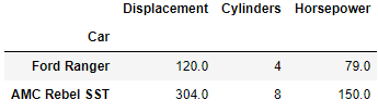
You can also output a DataFrame based on multiple row and column entries using loc.

df.loc[['Ford Ranger','AMC Rebel SST'],['Displacement','Cylinders','Horsepower']]

Using iloc

Single entries can be extracted from the DataFrame using iloc in the same manner as shown above with the loc method.

# extract the horsepower from the 4th row of the dataframe
>>> print(df.iloc[3,3])
150.0

DataFrame Slicing

DataFrames can be sliced in a similar manner to NumPy arrays and lists. Refer to our guides to list slicing and slicing of NumPy arrays if you need a refresher.

Slicing DataFrame Rows

Rows can be sliced directly by applying the slice condition to the DataFrame using square bracket notation.

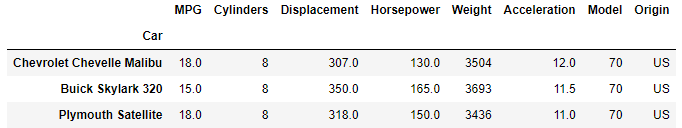
# slice the first three rows of the dataframe
df[0:3]

Slicing Rows and Columns

To extract a particular piece of the DataFrame when the row and column integer index number are known, use the iloc method.

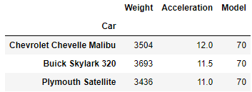
# select the last three columns of the first three entries
df.iloc[0:3,4:-1]

Slicing a DataFrame by Named Index and Columns

DataFrame slicing by name can be performed using the loc method. We have previously introduced this technique but it bears repeating here as this is a common operation performed when particular index and column names are known. The rows and columns do not need to be adjacent one-another when using this method.

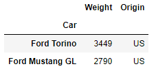
# using loc to slice a dataframe by name
df.loc[['Ford Torino','Ford Mustang GL'],['Weight','Origin']]

Wrapping Up

We've come to the end of our first article in a series of tutorials on pandas. In this post we have covered:

• Installation and setup.
• Series and Dataframe objects.
• Importing of raw data into a DataFrame from a CSV file.
• DataFrame slicing and the use of loc and iloc methods.

The next tutorial covers boolean indexing and DataFrame sorting. Hope to see you there!

Thanks for reading this tutorial and checking out CanardAnalytics. If you've enjoyed what you've seen and found our content helpful then please consider sharing it with your friends and colleagues as this is how we grow our audience and Python community.