
Linear algebra is the branch in mathematics that deals with linear equations and their representations in vector spaces through matrices. Matrix methods consist of a set of powerful tools used to work with linear systems, characterised by equations of the form:
$$a_{1}x_{1} + a_{2}x_{2}+a_{3}x_{3}+...a_{n}x_{n} = b$$
Linear algebraic methods are widely used in almost all areas of mathemmatics, and applied to many scientific and engineering applications. A good understanding of linear algebraic methods form a foundational element of any science, engineering or mathematics degree.
NumPy contains a very powerful linear algebra library which you will no doubt use extensively as you work with the package. This tutorial should serve as a guide and an introduction to some of the more commonly used functionality built into NumPy's linear algebra object.
Let's get started.
Scalar Dot Product
The dot product, or scalar product, is an operation that takes two equally sized array objects (such as a pair of coordinates), and returns a single scalar number.
Algebraically, the dot product of two vectors is the sum of the products of corresponding entries in the two vectors.
$$ a \cdot b = \sum_{i = 1}^{n} a_{i}b_{i} = a_{1}b_{1} + a_{2}b_{2} + a_{3}b_{3} + ... a_{n}b_{n} $$
The dot product is called in NumPy using the numpy.dot function.
numpy.dot(a, b, out=None)
To illustrate the dot product we will multiply two 2D cartesian coordinate vectors using the numpy.dot method and return a scalar value.
>>> import numpy as np

>>> coord1 = [1,4]
>>> coord2 = [3,5]
>>> dotproduct = np.dot(coord1,coord2)
>>> print(dotproduct)
23
The dot product also has a geometric interpretation when considering vectors in euclidean space. Namely the dot product of two vectors a and b is defined as the product of the magnitudes of each vector with the cosine of the angle between the vectors.
$$ a \cdot b = |a||b|\cos{\theta}$$
Referring to our example above, the dot product can then be determined geometrically as illustrated below.
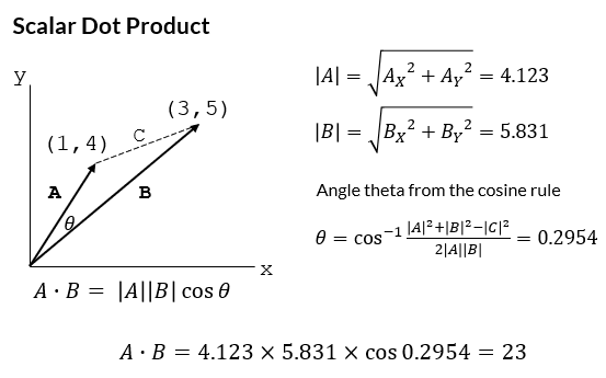
Combining the algebraic and geometric definitions of the dot product means that the angle between two vectors can be easily calculated by rearranging the geometric dot product formula:
$$\cos{\theta} = \frac{a \cdot b}{|a||b|}$$
I have personally used the formulation of the dot product to build an airport crosswind calculator where the angle between the prevailing wind and the runway in use must be determined before the parallel and crosswind components are calculated. This is a good example of a practical application of the dot product.
Matrix Cross Product
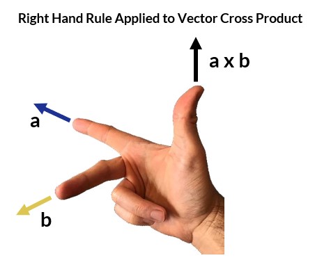
The cross product, or vector product, is a binary operation completed on two vectors, a and b, that results in a third vector that is perpendicular to a and b and thus normal to the plane containing them. The cross product is denoted by a × symbol.
The cross product has many applications in physics, engineering, and computer programming and is defined as follows:
$$a \times b = |a||b|\sin{(\theta})\textbf{n}$$
Where
- θ is defined as the angle between a and b in the plane containing them.
- |a| and |b| are the magnitudes of the two vectors.
- n is a unit vector perpendicular to the plane containing a and b.
The direction of the unit normal is given by the right hand rule, illustrated below.
The cross product is called in NumPy using the numpy.cross method.
numpy.cross(a, b, axisa=- 1, axisb=- 1, axisc=- 1, axis=None)
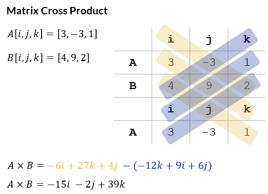
A cross product calculation is shown below specifying two 3D vectors.
# cross product of a 3D vector
>>> a = np.array([3,-3,1])
>>> b = np.array([4,9,2])
>>> cross = np.cross(a,b)
>>> print(cross)
[-15  -2  39]
The cross product can be manually calculated using matrix notation by making use of the Sarrus Rule illustrated below.
Calculating Moments Using the Cross Product
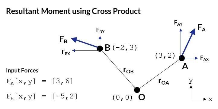
There are many fields within the sciences where the cross product finds a direct application. One such area is in the calculation of moments or torques — a common task in mechanical engineering.
The resulting moment M about a point O due to a due to an external force F applied some distance from O is determined by the cross product r × F.
$$ M_{O} = \vec{r_{OA}} \times \vec{F_{A}} $$
Let's run through an example now to show how we can quickly calculate the resultant moment acting at a given point by a set of external forces. What makes the cross product formulation of a moment calculation so powerful is that because the cross product obeys the right hand rule, the directions of the resulting moments are consistent through your calculation. This is very important if your are writing code to perform a moment calculation as you want a general solution that is applicable for any calculation setup.
Our example calculation requires that we calculate the resulting moment at point O from the two forces labelled FA and FB.
- The cartesian coordinates of points O, A, and B are given in the sketch below.
- The force components in the x and y directions are also given.
The calculation steps are as follows:
- Calculate the distance vectors from the origin (point O) to the applied external forces (points A and B).
- Add these to a NumPy array containing the postion vectors of all the external forces.
- Create a NumPy array to house the external forces.
- Perform the cross product using the
np.crossmethod. - The result will be an array of the moment contribution from each external force acting at point O.
- Sum these together to arrive at the total moment acting at O from all forces.
This can be implemented in Python as follows:
import numpy as np

# moment calculation using the cross product
# coordinates of points in model
O = [0,0]
A = [3,2]
B = [-2,3]

# force components at point A and B
FA = np.array([[3,6]]) # [x,y]
FB = np.array([[-5,2]])

def posvector(origin,a):
    """ return a position vertor between
        and two coordinate points.
    """
    vec = np.subtract(a,origin)
    return np.array([vec])

rOA = posvector(O,A)
rOB = posvector(O,B)

# create the position and force arrays
r_array = np.concatenate((rOA,rOB),axis=0)
F_array = np.concatenate((FA,FB),axis=0)

MO = np.sum(np.cross(r_array,F_array)) # cross product and sum
print(f"The total moment about point O is {MO}.")
Running through the script above will print out the resulting moment.
"The total moment about point O is 23."
You can validate the Python script and result with your own hand calculation.
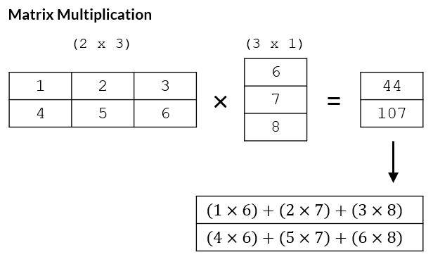
Matrix Multiplication
Matrix multiplication is an operation that produces a single matrix from two input matrices, and can only be performed if the number of columns in the first matrix is equal to the number of rows in the second matrix.
The resulting matrix will have a size equal to the number of rows of the first matrix, and the number of columns of the second.
The product of two matrices A and B is denoted AB.
Matrix multiplication in NumPy is performed using the numpy.matmul method. It is a very common operation to perform in NumPy and as such a shorthand operator @ has been specified since PEP465 to improve readibility and in the words of the PEP465 release, "provides a smoother onramp for less experienced users, who are particularly harmed by hard-to-read code and API fragmentation."
>>> A = np.array([[1,2,3],[4,5,6]])
>>> B = np.array([6,7,8])

>>> AB = np.matmul(A,B)
>>> print(AB)
[ 44 107]
# the @ symbol is shorthand for numpy.matmul
>>> AB2 = A @ B
>>> print(AB2)
[ 44 107]
>>> print(AB2.shape)
(2,)
If A is an m x n matrix and B is a n x p matrix then the matrix product C = AB is an m x p matrix defined as:
$$c_{ij} = a_{i1}b_{1j} + a_{i2}b_{2j} + ... + a_{in}b_{nj} = \sum_{k=1}^{n} a_{ik}b_{kj} $$
This may be clearer when provided with an example. The matrix multiplication in the code block above is illustrated below showing how the multiplication is performed.
Determinate and Inverse
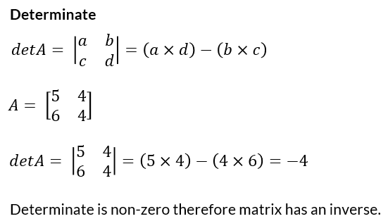
Matrix Determinate
The determinate of a square matrix is a scalar value that provides some insight into the characteristics of that matrix. Principally, the determinate of a matrix is non-zero if and only if that matrix has an inverse.
Knowing whether or not a matrix has an inverse is very useful when solving a set of linear equations using matrix methods in the form:
$$\textbf{A}\textbf{x} = \textbf{b}$$
The determinate is calculated in NumPy with the function numpy.linalg.det.
>>> import numpy as np
>>> A = np.array([[5,4],[6,4]])
>>> print(np.linalg.det(A))
-4 # non-zero therefore inverse exists
Matrix Inverse
An n x n square matrix A is said to be invertible (has an inverse) if there exists a square n x n matrix B such that
$$\textbf{AB} = \textbf{BA} = \textbf{In}$$
where In is an n x n identity matrix (1's on the main diagonal, zeros elsewhere).
The matrix inverse is found in NumPy using the np.linalg.inv function.
>>> A = np.array([[5,4],[6,4]])
>>> Ainv = np.linalg.inv(A)
>>> print(Ainv)
[[-1.    1.  ]
 [ 1.5  -1.25]]

# now multiply A and Ainv to show the identity matrix
>>> ident = A @ Ainv
>>> print(ident)
[[ 1.0000000e+00 -8.8817842e-16]
 [ 0.0000000e+00  1.0000000e+00]]
We can further illustrate the relationship between the determinate and the inverse by writing a simple function that will calculate the determinate of an input matrix, and then invert the matrix if and only if the matrix has a non-zero determinate.
# matrix determinate
# The determinate of a non-zero matrix is invertible
a1 = np.array([[3,4],[6,8]])
a2 = np.array([[5,4],[6,4]])
a3 = np.array([[5,4,2],[6,4,1],[5,7,9]])

def detInverse(a):
    deta = np.linalg.det(a)
    if deta != 0:
        inva = np.linalg.inv(a)
    else:
        inva = None
    return deta,inva
The results for the three matrices a1, a2, a3:
print(detInverse(a1))
(0.0, None) # determinate zero - no inverse matrix

print(detInverse(a2))
(-3.999999999999999, # determinate -4
array([[-1.  ,  1.  ], # inverse matrix
       [ 1.5 , -1.25]]))

print(detInverse(a3))
(-7.000000000000009, # determinate -7
 array([[-4.14285714,  3.14285714,  0.57142857], # inverse matrix
       [ 7.        , -5.        , -1.        ],
       [-3.14285714,  2.14285714,  0.57142857]]))
As mentioned at the start of this section, inverting a square matrix is a fundamental step in solving for a set of linear equations. Let's move onto this next.
Solving a System of Linear Equations
A system of linear equations is a collection of one or more linear equations that contain the same variables. You may be more familiar with the terminology of simultaneous equations — this is the same thing.
To solve a system of linear equations requires that the number of equations used to define the system is equal to the number of unknowns in the system.
Matrix methods lend themselves very nicely to solving such a set of linear equations. We'll demonstrate the theory and then how to go about solving a system using NumPy.
Theory of Linear Systems
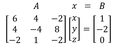
Consider the system defined by the set of linear equations shown below. There are three unknowns, x, y, z, and three equations.
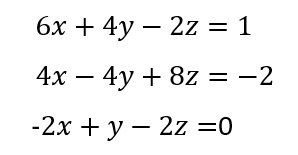
In order to solve these equations using matrix methods we must rewrite the equations in the form:
$$\textbf{A}\textbf{x}=\textbf{B}$$
x is a column of the unknowns, A is a matrix of the coefficients of the unknowns, and B is a matrix of the constants (RHS).
We wish to solve for x, which we can do by multiplying the LHS and RHS of the matrix system by the inverse of the A matrix.
$$A^{-1}Ax=A^{-1}B$$
$$x = A^{-1}B$$
Performing the matrix inversion and subsequent matrix multiplication yields the following result:
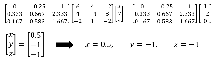
We have therefore solved the three unknowns efficiently using matrix methods.
Solving Linear Systems using NumPy
Performing this calculation in Python using NumPy is significantly easier than doing it by hand. First you need to define your NumPy arrays (A and B matrix), whereafter you invert the A matrix and multiply the inverse A by B. The script below performs these actions and prints of the results.
import numpy as np
A = np.array([[6,4,-2],[4,-4,8],[-2,1,-2]])
B = np.array([1,-2,0])
Ainv = np.linalg.inv(A) # invert A
x = np.matmul(Ainv,B) # multiply A^-1 by B
print(f"[x,y,z] = [{x[0]},{x[1]},{x[2]}]")
The results are printed out below:
[x,y,z] = [0.5,-1.0,-1.0]
Solving Linear Systems with np.linalg.solve
The calculation performed above is so common that rather than having to manually call numpy.linalg.inv and numpy.matmul you can just use the predefined numpy.linalg.solve function which performs the inversion and multiplication in the background.
import numpy as np
A = np.array([[6,4,-2],[4,-4,8],[-2,1,-2]])
B = np.array([1,-2,0])
x = np.linalg.solve(A,B) # calls the solve routine
print(f"[x,y,z] = [{x[0]},{x[1]},{x[2]}]")
The output:
[x,y,z] = [0.5,-1.0,-1.0]
Real World Example: Forces on a Control Arm
It's always nice to show a real-world application when describing how to perform a particular type of analysis or calculation. Let's use the linear system solver described above to determine the reaction loads exerted on a control arm due to a loading input.
Refer to the picture below showing a control arm with two external forces applied to it. The arm pivots about point O and will react the external loading at point O and at point A.
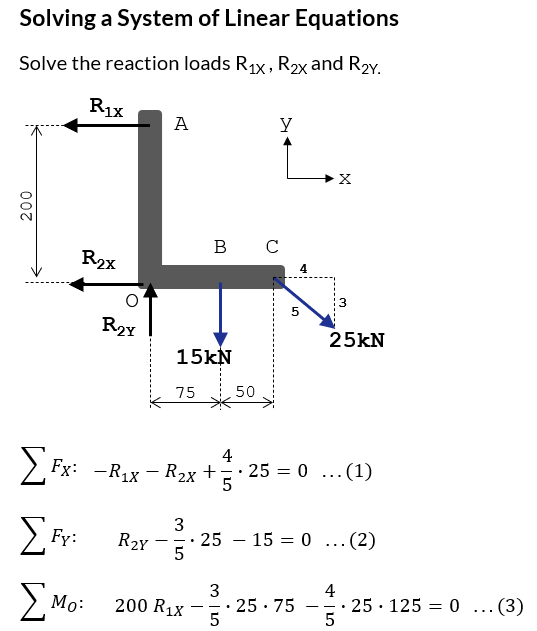
There are three unknown reaction forces (R1x, R2x, R2y) and so three equations must be generated to describe the system in order to solve for these unknown reactions. Since the control arm is in equilibrium,
- Sum of forces in the x-direction must equal zero.
- Sum of forces in the y-direction must equal zero.
- Sum of moments at O must equal zero.
This is therefore a linear system and can be represented by the matrix notation:
$$\textbf{A}\textbf{x}=\textbf{B}$$
Which can be solved using numpy.linalg.solve as we did before.
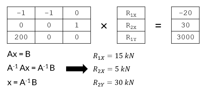
The Python code looks as follows:
import numpy as np
a = np.array([[-1,-1,0],[0,0,1],[200,0,0]])
b = np.array([-20,30,3000])

x = np.linalg.solve(a,b)
print(f"Resultant Forces: R1x = {x[0]} kN, R2x = {x[1]} kN, R2y = {x[2]} kN.")
Running the script above will print out the resulting three forces.
"Resultant Forces: R1x = 15.0 kN, R2x = 5.0 kN, R2y = 30.0 kN."
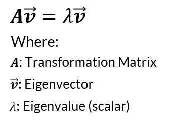
Eigenvalues and Eigenvectors
We'll end this tutorial off with a quick look at NumPy's eigenvalue and eigenvector routines. We won't delve too deeply into the theory behind eigenvectors and eigenvalues suffice as to say,
- An eigenvector of a linear transformation is a non-zero vector that changes at most by a scalar factor when a linear transformation is applied to it.
- The corresponding eigenvalue is the factor by which the eigenvector is scaled.
This is represented in mathematically as:
If you'd like a more detailed explanation of eigenvectors and eigenvalues then the YouTube channel 3Blue1Brown has an excellent video that goes over the theory in great detail.
NumPy provides the numpy.linalg.eig function to work with eigenvalues and eigenvectors. The function returns a tuple.
- The first entry is an array of eigenvalues,
- The second entry is an array of eigenvectors.
Let's run through a simple example where we'll generate the eigenvalues and eigenvectors for a 2 x 2 matrix.
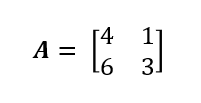
Our Python script to extract eigenvalues and eigenvectors looks as follows:
>>> import numpy as np
>>> A = np.array([[4,1],[6,3]])
>>> eig1 = np.linalg.eig(A)
>>> print(eig1)
(array([6., 1.]),
 array([[ 0.4472136 , -0.31622777],
       [ 0.89442719,  0.9486833 ]]))
Matrix A has two eigenvalues, 6 and 1.
The eigenvectors corresponding to each eigenvalue are extracted from the two columns in the eigenvector array.
# print eigenvector 1
>>> eigvalue1 = eig1[0][0]
>>> print(eigvalue1)
6.0
>>> eigvector1 = eig1[1][:,0]
>>> print(eigvector1)
[0.4472136  0.89442719]

# print eigenvector 2
>>> eigvalue2 = eig1[0][1]
>>> print(eigvalue2)
1.0
>>> eigvector2 = eig1[1][:,1]
>>> print(eigvector2)
[-0.31622777  0.9486833]
Wrapping Up
This has been a busy tutorial and we have covered a lot of ground. Let's reflect on what we have worked through.
- We started by looking at the Scalar Dot Product and its definition, both algebraically and geomtrically.
- We covered the Matrix Cross Product and used this to calculate moments around a point in 2D space.
- We looked at Matrix Multiplication
numpy.matmuland the shorthand operator@. - We showed how the Determinate may be used to determine whether a matrix is invertible or not, and then looked more closely at Matrix Inversion.
- We then took everything we have learned and applied it to solving a system of linear equations in NumPy. The function
numpy.linalg.solveperforms this without us having to manually invert and multiply the matrices. - Finally we briefly touched on Eigenvectors and Eigenvalues, and how NumPy handles them with the
numpy.linalg.eigmethod.
Thanks for sticking around to the end. Linear algebra is a fundamental concept in the mathematics and science industries, and NumPy can make working on these sometimes complicated concepts much easier. If you did find this tutorial valuable then please share it with others, this will help us to continue to build our Python community!