Boolean Indexing and Sorting in Pandas

Introduction

Pandas is a powerful data analysis and manipulation software library, and has become one of the de-facto standard packages used whenever analytical analysis is performed on large datasets in Python. This is part two in our pandas series where we cover boolean indexing and DataFrame sorting. In part one we covered setup, the DataFrame and Series objects, importing raw data from a CSV file, and some DataFrame slicing and selection.

The primary focus of this tutorial is boolean indexing which involves applying conditional statements to a parent DataFrame, filtering and extracting information in such a way as to provide new insight into our dataset.

Sample Dataset

We'll make use of the same classic car dataset that we did in the first pandas tutorial. The dataset was originally sourced from Kaggle and is available to download here.

Remember that the pandas package must be installed in your Python distribution before you can use it to perform any analysis. Once installed you need to import the package into your script or notebook in order to access its methods, classes, objects, or functions. Most scientific Python distributions like Anaconda come prebundled with pandas and this is the recommended way to setup and use the library. If you are unsure how to do this then refer to the installation section in the first tutorial.

In keeping with convention we import pandas using the abbreviation pd.

import pandas as pd

Read the downloaded CSV file into a new DataFrame using the read_csv method and set the index to the "Car" column. I have made use of the os module (import os) to correctly build my file-path, but this is not necessary if the CSV file and your script/notebook are housed in the same folder.

folder = 'imports'
filename = 'classic-cars.csv'
path = os.path.join(folder,filename)

df = pd.read_csv(path,index_col='Car')

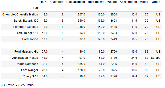
Displaying the newly created DataFrame shows that we have 8 columns that describe a number of classic cars, and 406 rows representing different vehicles.

We now have everything in place to begin filtering our dataset by boolean indexing.

Boolean Indexing

Boolean indexing refers to filtering data in a DataFrame through the creation of a boolean vector of equal dimension to the DataFrame being filtered. Put another way, you can apply a set of comparison and boolean operators (and, or, not) to a DataFrame, which will operate on that dataFrame and only return row and column entries where the resulting conditional returns True.

This is a powerful and convenient way to reduce your data in order to provide meaningful results and insight.

The valid comparison operators are:

• >, <, >=, <=, ==

  and boolean operators:

• Use & for boolean and,
• Use | for boolean or,
• Use ~ for boolean not.

We'll start with filtering by a simple single conditional and progress from there to more complex multiple conditional statements.

Single Conditional

A single conditional operation is performed on a DataFrame column using square bracket notation. Take a look at the code shown below where we have printed out a boolean series where True is assigned to all rows where the fuel consumption 'MPG'  is greater than 40 miles per gallon.

The resulting series is equal in length to the number of rows in the DataFrame.

>>> print(df['MPG']>40)
"""
Car
Chevrolet Chevelle Malibu    False
Buick Skylark 320            False
Plymouth Satellite           False
AMC Rebel SST                False
Ford Torino                  False
                             ...  
Ford Mustang GL              False
Volkswagen Pickup             True
Dodge Rampage                False
Ford Ranger                  False
Chevy S-10                   False
Name: MPG, Length: 406, dtype: bool
"""

Filtering of the original DataFrame is performed by passing the boolean series just created to the full DataFrame through square bracket notation.

fuel_efficient = df[df['MPG']>40]

The DataFrame is then filtered by that condition and only rows where the MPG is greater than 40 are added to the new DataFrame named fuel_efficient here.

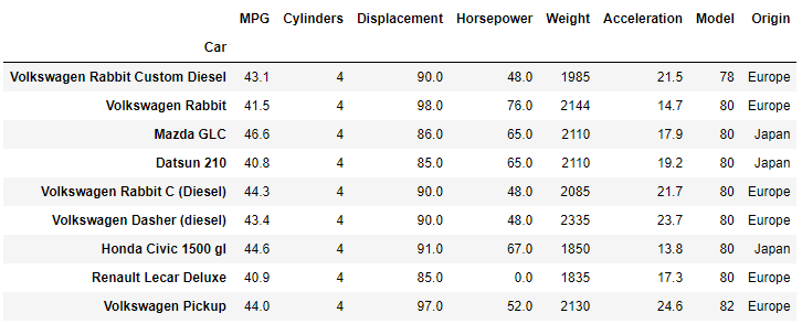
The result is shown above and the original DataFrame with 406 different car entries (rows) has been reduced to only 9 remaining entries. Two interesting conclusions can immediately be drawn from the resulting dataset: (i) there are no US vehicles in the list and (ii) all vehicles remaining have 4 cylinder engines.

Multiple Conditionals

As soon as you have more than one conditional that must be satisfied you start working with boolean operators. It is very important that the operators are grouped using parentheses in order to ensure that expresions are evaluated correctly. We'll cover a few examples to show the importance of bracketing correctly.

Multiple Conditions AND

Our first example is a simple AND statement where we are looking to filter by european cars with six or more cylinders. The syntax for the conditional is shown below. 

EUcars = df[(df['Origin']=='Europe') & (df['Cylinders']>=6)]

There are only four cars in our dataset that meet both conditions.

Multiple Conditions OR

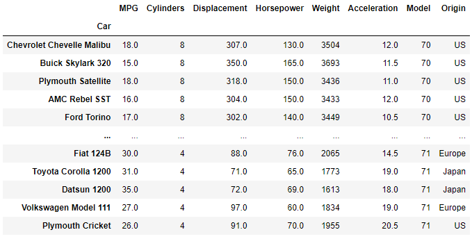
Let's now filter our dataset to only include car models from 1970 and 1971.

# multiple conditions boolean OR
old_cars = df[(df['Model']==70) | (df['Model']==71)]

Multiple AND and OR Conditionals

Careful bracketing is particularly important when working with more than two conditional statements. We now wish to filter our dataset to only show Japanese car models from 1970 or 1971.

Note the double brackets enclosing the or operator which serves to perform that operation in isolation of the first condition and apply it as a single result to the and condition of the vehicles being Japanese.

# japanese cars with year model 1970 or 1971
japan_old_cars = df[(df['Origin']=='Japan') & ((df['Model']==70) | (df['Model']==71))]

The result is six vehicles that meet our criteria.

If you neglect the brackets housing the or statement the expression will be incorrectly interpreted as:

1. filter by Japanese cars from 1970,
2. or any vehicle from 1971.

This will result in a completely different dataset being returned which highlights the importance of carefully considering the filtering conditions and subsequent bracketing before finalising the analysis.

Indexing by isin

Another means of boolean indexing is the Series.isin() method. This returns a boolean series showing whether each element in the series exactly matched an element in the passed sequence of values.

Since this works on a Series we generally apply the method to a column with one or more acceptable values as input.

We can use isin to filter our dataset by 1972 model vehicles with exactly 150.0 HP engines. 

# 150 HP cars manufactured in 1972
HPcars1972 = df[(df['Horsepower'].isin([150.0])) &  (df['Model'].isin([72]))]

The result is four cars that meet this criteria.

If we wished to extend our filtering to include car models from 1973 we could simply add that model year to that isin list.

new_criteria = df[(df['Horsepower'].isin([150.0])) &  (df['Model'].isin([72,73]))]

Indexing by isna

Very often a dataset will consist of entries that are NA. These are values such as None, numpy.NaN, or numpy.NaT. You can quickly filter these out using the Series.isna method.

If we apply this method to our filtered list of cars from 1972 with 150.0 HP we are returned a DataFrame where every entry is False. 

HPcars1972.isna()

Sorting Values

Once a dataset has been filtered using the methods described above, it is common to then sort the resulting DataFrame by one (or more) of the columns to aid in the interpretation of the result.

The sorting is performed through the sort_values method.

DataFrame.sort_values(by, axis=0, ascending=True, inplace=False, kind='quicksort', 
                      na_position='last', ignore_index=False, key=None)

• by refers to a string or list of strings with the names by which to sort. Often you will sort by a single column and by refers to that column name.
• axis refers to the DataFrame axis to sort. 0 refers to the index and 1 to the columns. The default is 0 which will sort the DataFrame rows by the columns listed in by.
• You can choose whether to sort by ascending (default) or descending order with the ascending parameter. If you are sorting by multiple columns or rows (a list in the by parameter) then you need a list of booleans of equal length to assign the ascending parameter.

Refer to the official API documentation for further information on the other parameters not covered here. The sorting methods available are the same as those in numpy.sort. 

Single Sort Parameter

Let's run through a worked example where the sort_values method is applied after a boolean indexing opertion.

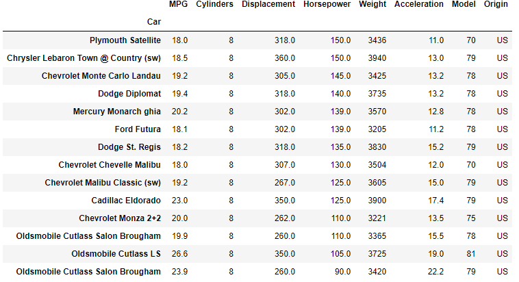
Starting with our original classic cars DataFrame we'll first generate a new DataFrame of US 8 cylinder cars with a fuel consumption of 18 MPG or greater, and then order the resulting list from most powerful (highest HP) to least powerful.

We can achieve this in a single step, combining what we have learnt about boolean indexing with the sort_values method.

# US cars with 8 cylinders and fuel consumption 18 MPG or better
# sort by HP in descending order
UScars_8cyl = df[(df['Origin']=='US') & (df['Cylinders']==8) & 
                 (df['MPG']>=18)].sort_values('Horsepower',ascending=False)

The resulting DataFrame is now conveniently sorted by horsepower.

Multiple Sort Parameters

Since there are a few cars in our resulting DataFrame with the same power output we may wish to sort by more than one column. To do this requires a modification to the by attribute and the ascending attribute in our sort_values call.

We'll now sort by two criteria:

1. First sort by Horsepower in descending order.
2. Then sort by Model in descending order (latest model first).

The modified code looks as follows:

sortby = ['Horsepower','Model']
sort_direction_list = [False,False]

twosort = df[(df['Origin']=='US') & (df['Cylinders']==8) & 
             (df['MPG']>=18)].sort_values(by=sortby,ascending=sort_direction_list)

To sort by multiple criteria simply pass a list of column names to sort by to the by parameter, and a list of booleans of equal length to the ascending parameter to determine the direction of the sorting. 

The final sorted DataFrame now looks as follows:

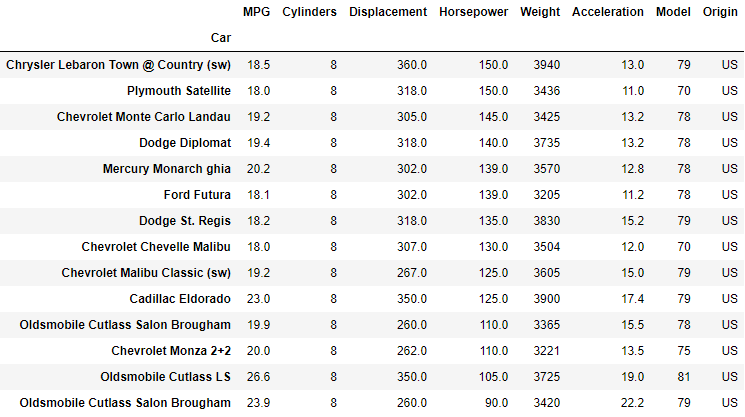
The first two entries have been swapped around to match our new criteria as well as a few others further down the list.

Wrapping Up

This brings us to the end of our second tutorial on pandas. Here we have built on from what was learnt in the first pandas tutorial and subsequently covered:

• Boolean indexing to filter DataFrames by comparison and boolean operators.
• Indexing using the isin and isna methods.
• Sorting of DataFrames using the sort_values method.

Our next tutorial covers grouping using the groupby method and the creation of pivot tables. Hope to see you there!

Thanks for reading this CanardAnalytics tutorial. If you've enjoyed what you've read, and found the content helpful then please consider sharing it with your friends and colleagues as this is how we grow our audience, and the Python community at large.