If you are plannnig to work with numerical data in Python (as you almost certainly are) then NumPy quickly becomes an essential tool in your toolkit. This tutorial is the first in a series on NumPy and serves as an introduction to this popular Python package.
What is NumPy
NumPy (Numerical Python) is a scientific computing package centered around the multidimensional array object which enables you to perform fast and efficient array and matrix opertations within your Python codebase. NumPy ships with a large assortment of routines to facilitate all the matrix and array operations you could every wish to perform: including, but not limited to, mathematical operations, sorting and shape, logical, statistical, linear algebra and random simulation. As soon as you start to work with larger data sets in Python, or any scientific or engineering application, NumPy quickly becomes an essential component of your codebase.
Installation
NumPy is a Python package that must be installed before use. Installation can be completed through conda or pip. However, many scientific Python distributions are available which will all come preinstalled with NumPy, and this is the preferred way to quickly get up and running, as many of the other commonly used data science packages will also be bundled in the install.
Two commonly used scientific distributions are Anaconda and WinPython.
If you need additional help getting NumPy installed on your Python distribution then head over to the NumPy Installation Guide before continuing with this tutorial.
Once you have the NumPy package installed then don't forget to import it. The convention is to refer to NumPy using the abbreviation np.
import numpy as np
Why Choose NumPy Over Python Lists
The short answer is speed and ease of use. NumPy performs all looping and indexing in the background using pre-compiled C code. When working with NumPy you shouldn't be setting up your own for loops to iterate through the arrays - by default NumPy works on element-by-element operations. This allows you to write very clean and Pythonic code which is significantly faster to execute over a standard Python iterable; especially when very large datasets are being worked on.
A good example of the simplicity that NumPy brings to working with numerical data can be illustrated by multiplying each element in 1-D array with a corresponding element in another 1-D array of equal dimensions. Compare how this is achieved using Python lists, and the equivalent NumPy code.
# List implementation of the code
c = []
for i in range(len(a)):
    c.append(a[i]*b[i])

# NumPy implementation of the code
c = a * b
NumPy Multidimensional Array Object
At the core of the NumPy package is the numpy.ndarray class which is known by its alias numpy.array. A NumPy array is a homogenous multidimensional table of elements indexed by a tuple of non-negative integers.
The dimensions of the array are referred to in NumPy as axes. A vector or coordinate in three-dimensional space, [3,6,8], has a single dimension and therefore one axis. There are three elements in the axis corresponsing to the x,y,z coordinate points. We therefore say that the coordinate point has one axis and a length of three.
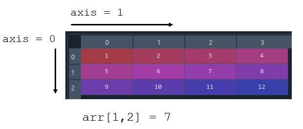
A two-dimensional array (2-D matrix) has two axes and two lengths, equal to the number of elements in each axis. The example array below has two axes and a length of (3,4) corresponding to to the number of rows and columns respectively. Indexing of elements in the array start at zero and are accessed using square brackets with convention arr[row,col].
Creating Arrays
There are a number of different ways to create a NumPy array. We'll start by looking at the np.array() method which takes a list or tuple as an input and outputs a numpy.array. Thereafter we'll explore some other ways to create more specific arrays; for example we can easily create an array of zeros or ones.
One Dimensional Arrays
One dimensional arrays have a single axis, and a length equal to the number of elements in the array. Arrays are most often created using a list as the input parameter.
numpy.array(object, dtype=None, *, copy=True, order='K', subok=False, ndmin=0, like=None)
Let's create a simple 1D array now.
import numpy as np
arr = np.array([1,2,3,4])
We can print the number of dimensions by calling .ndim and a tuple corresponding to the number of rows and columns with .shape.
>>> print(arr)
[1 2 3 4]
>>> print(arr.ndim) # number of dimensions
4
>>> print(arr.shape) # number of (rows,cols)
(4,)
Two Dimensional Arrays
Two dimensional arrays are created using nested lists or nested tuples. The array method transforms sequences of sequences into two-dimensional arrays and sequences of sequences of sequences into three-dimensional arrays, and so on.
Consider the 3 x 4 matrix (array) shown below.
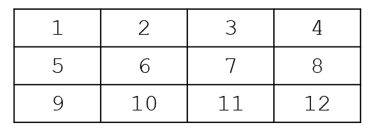
This is generated as a NumPy array as follows:
import numpy as np
arr2d = np.array([[1,2,3,4],[5,6,7,8],[9,10,11,12]])
>>> print(arr2d)
[[ 1  2  3  4]
 [ 5  6  7  8]
 [ 9 10 11 12]]
>>> print(arr2d.ndim)
2
>>> print(arr2d.shape)
(3,4)
Higher Order Arrays
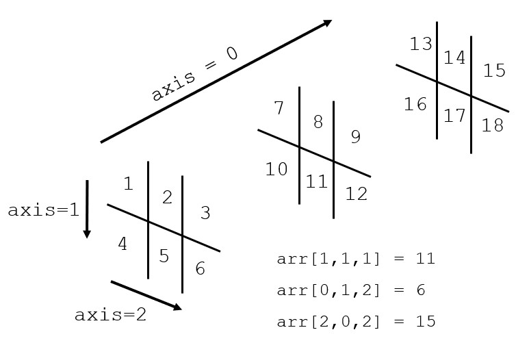
Higher order arrays are created by a further nesting of lists. A three-dimensional array is shown below as an example.
arr3d = np.array([[[1,2,3],[4,5,6]],[[7,8,9],[10,11,12]],[[13,14,15],[16,17,18]]])
>>> print(arr3d)
[[[ 1  2  3]
  [ 4  5  6]]

 [[ 7  8  9]
  [10 11 12]]

 [[13 14 15]
  [16 17 18]]]
>>> print(arr3d.ndim)
3
>>> print(arr3d.shape)
(3,2,3)
This 3D array can be thought of as three 2 x 3 matrices, drawn below with axes labelled for clarity.
Axis and Shape of Arrays
The examples above have already introduced the concept of number of dimensions (axes) and the shape of the array. We can extract these from our arrays using the ndim and shape attributes respectively.
>>> arr2d = np.array([[1,2,3,4],[5,6,7,8],[9,10,11,12]])
>>> print(arr2d.ndim)
2
>>> print(arr2d.shape)
(3,4)
Additional Array Creation Methods
There are a number of other methods you can use to create NumPy arrays. We'll go over some of these now and explain when you may wish to use them.
Array of Zeros
You can define an array of any dimension filled with zeros using the numpy.zeros function. The input is a tuple containing the dimensions of the desired array. The default data type is float64, but this can be modified with the dtype parameter.
numpy.zeros(shape, dtype=float, order='C', *, like=None)
>>> arr_zero = np.zeros((3,4))
>>> print(arr_zero)
[[0. 0. 0. 0.]
 [0. 0. 0. 0.]
 [0. 0. 0. 0.]]
Array of Ones
An array of ones is identical to the np.zeros method except that the resulting array will be filled with ones rather than zeros.
>>> ones = np.ones((2,3),dtype=int)
>>> print(ones)
[[1 1 1]
 [1 1 1]]
Creating an array of zeros or ones is very useful when you need to initialise an array so long as the dimensions are known. Once created, you can then populate the array with a set of calculated values. In this instance the array of ones or zeros simply acts as a container.
Arange
This is very similar to the Python range function which allows you to create a 1D array with regular incrementing (evenly spaced) intervals.
numpy.arange(start, stop, step, dtype=None, *, like=None)
The start parameter is included in the range and the stop parameter is excluded. It's best to use integer start, stop and step values when working with arange. Linspace is preferred if you need to step in fractions as you can guarentee the number of increments without worry of rounding errors.
>> myrange = np.arange(2,9,2) # incl start but exclude stop
>> print(myrange)
[2 4 6 8]
Linspace
This will return evenly spaced numbers over a specified interval. This differs from arange in that rather than specifying the step, here you specify the number of intervals.
numpy.linspace(start, stop, num=50, endpoint=True, retstep=False, dtype=None, axis=0)
By default the value given in stop will be included in the resulting 1D array, Defining endpoint=False will exclude the stop value.
>>> lin1 = np.linspace(0,10,num=6,endpoint=True)
>>> print(lin1)
[ 0.  2.  4.  6.  8. 10.]

>>> lin2 = np.linspace(0,10,num=6,endpoint=False)
>>> print(lin2)
[0. 1.66666667 3.33333333 5. 6.66666667 8.33333333]
Empty Arrays
The function empty creates an array of a specified size, filled with random content which is dependent on the state of the memory. You may prefer to use numpy.empty if you need to initialize a very large array, as it is faster than using numpy.zeros or numpy.ones. Just remember that if you do create an empty array the element values are random and must be overwritten later to avoid some strange results.
numpy.empty(shape, dtype=float, order='C', *, like=None)
emp1 = np.empty((3,4)) # 3 x 4 array of random content
Sorting Arrays
Ordering or sorting arrays of data is a very common numerical task. This is easy to complete when using the numpy.sort() function.
The Sort Method
The sort() function takes the following parameters:
numpy.sort(a, axis=- 1, kind=None, order=None)
Where a is array to sort. The axis parameter sets the axis along which the array will be sorted. The default sorts the array along the last axis. The sorting algorithm can also be modified using the kind parameter. Sorting is performed in ascending order.
Sort and Flattern
To flattern the array when sorting add axis=None to the sort call.
>>> arr1 = np.array([[31,4,5],[2,1,4],[8,9,7]])
>>> arr2 = np.sort(arr1,axis=None) #flattern array
>>> print(arr2)
[ 1  2  4  4  5  7  8  9 31]
Sort Each Row
To sort each row of a 2D array in ascending order you need to specify the axis along which to sort. In this case we need to sort along axis=1.
>>> arr2sort = np.array([[6,3,7,4,6,9],[2,6,7,4,3,7],[7,2,5,4,1,7],[5,1,4,0,9,5]])
>>> print(arr2sort)
[[6 3 7 4 6 9]
 [2 6 7 4 3 7]
 [7 2 5 4 1 7]
 [5 1 4 0 9 5]]

>>> rowsorted = np.sort(arr2sort, axis=1)
>>> print(rowsorted)
[[3 4 6 6 7 9]
 [2 3 4 6 7 7]
 [1 2 4 5 7 7]
 [0 1 4 5 5 9]]
It's important to remember that as soon as you are sort by row (or column) the entries become independent of eachother and any relationships between entries in rows or columns are lost.
Sort Each Column
This works in the same way as row sorting except that now you are sorting along axis=0.
>>> arr2sort = np.array([[6,3,7,4,6,9],[2,6,7,4,3,7],[7,2,5,4,1,7],[5,1,4,0,9,5]])
>>> print(arr2sort)
[[6 3 7 4 6 9]
 [2 6 7 4 3 7]
 [7 2 5 4 1 7]
 [5 1 4 0 9 5]]

>>> colsorted = np.sort(arr2sort, axis=0)
>>> print(colsorted)
[[2 1 4 0 1 5]
 [5 2 5 4 3 7]
 [6 3 7 4 6 7]
 [7 6 7 4 9 9]]
Modifying the Sorting Algorithm
There are four different sorting algorithms that you can employ when using sort, selected using the kind parameter.
kind = {'quicksort','mergesort','heapsort','stable'}
The default is quicksort which should suffice for most cases.
ArgSort Method
The argsort method is used if you want an output of the order of indices that would sort the array rather than the array itself. Other than the output, argsort works in the same way as sort and allows you to sort by row, column, or flattern the array. You can output the sorted array (values) using square bracket notation as illustrated in the example below.
>>> arr2sort = np.array([5,7,8,9,9,0,3])
>>> print(arr2sort)
[5,7,8,9,9,0,3]

>>> sorted_idx = np.argsort(arr2sort)
>>> print(sorted_idx)
[5 6 0 1 2 3 4] # this is an array of indexes corresponding to the original array

# you can retrieve a sorted array as follows
>>> sorted = arr2sort[sorted_idx]
>>> print(sorted)
[0 3 5 7 8 9 9]
Array Partitioning
There may be cases where you need to extract the value of the k-th element in a sorted array. You can of course simply sort the array and then extract the k-th element, but for large datasets this is computationally inefficient as you don't actually need to sort the entire dataset, you just need the one element in the correctly sorted position.
In these instances it is better to use the numpy.partition() function.
numpy.partition(a, kth, axis=- 1, kind='introselect', order=None)
This function will return a copy of array a with its elements rearranged in such a way that the value of the element in the k-th position is in the position it would be in if it were in a sorted array.
A few things to note:
- All elements smaller than the k-th element are moved before this element.
- All elements greater or equal to the k-th element are moved after.
- The ordering of the elements in the two partitions are undefined.
The default value for axis is -1, which will sort the array along the last axis. You can specify the axis to sort along in the same way as you do with the numpy.sort function. You can also set axis = None to flatten the array.
# example using numpy.partition
# partition allows you to extract the nth smallest values in the array.
# Note that the array is split into two partitions. Neither partition is sorted.
>>> arr_raw = np.array([5,1,6,22,9,4,100,3,2,23,54,89,17,11,445])
>>> print(arr_raw)
[  5   1   6  22   9   4 100   3   2  23  54  89  17  11 445]
>>> partition_at = 5 # select the nth item to partition
>>> arr_part = np.partition(arr_raw,partition_at)
>>> print(arr_part) # partitioned array
[  4   3   2   1   5   6   9  11  17  22  23  89  54 100 445]
Array Concatenation
NumPy's concatenation function provides a powerful method to join sequences of arrays along an existing axis. Simply put, if you need to build up a matrix from a set of smaller arrays, then use numpy.concatenate() to do this quickly and efficiently.
numpy.concatenate((a1, a2, ...), axis=0, out=None, dtype=None, casting="same_kind")
The arrays that you wish to join must be passed to the function as a tuple. The axis parameter defines along with axis or dimension the arrays should be joined. The default axis=0 will join on the zero axis. You can also specify axis=None to flatten all the arrays.
Concatenating arrays is a very common task and so we'll run through a few examples where we join two 2-D arrays along various axes.
For all our examples we'll use the two matrices given below.
a = np.array([[1, 2], [3, 4]]) # 2 x 2 matrix
b = np.array([[5,6]]) # 1 x 2 matrix
Flatten
To flatten the resulting array we set axis=None on our numpy.concatenate call.
>>> c1 = np.concatenate((a,b),axis=None) # None flattens the arrays
>>> print(c1)
[1 2 3 4 5 6]
Concatenation of Rows
To concatenate along the rows axis we set axis=0. This will add array b as a new row below array a.
>>> c2 = np.concatenate((a,b),axis=0) # adding a new row
>>> print(c2)
[[1 2]
 [3 4]
 [5 6]]
>>> print(c2.shape)
(3, 2)
Concatenation of Columns
Concatenation of columns requires that we transpose array b from a 1 X 2 matrix to a 2 X 1 matrix. The axis is set to 1 to add the transposed matrix to array a as a new column.
>>> c3 = np.concatenate((a,b.T),axis=1) # here we must transpose the matrix B.
>>> print(c3)
[[1 2 5]
 [3 4 6]]
>>> print(c3.shape)
(2, 3)
Summary
We've come to the end of this introduction to the NumPy package where we covered the following topics.
- We explained why NumPy is far more powerful than native Python lists when working with numerical datasets.
- The creation of multidimensional NumPy arrays from Python iterables (most often lists).
- Described the size and shape of arrays and how to access that information.
- We looked at other methods for array creation.
- The creation of an array of zeros or ones.
- Looked at the difference between
arangeandlinspacewhen creating 1-D arrays.
- Worked through array sorting methods, and showed how setting the
axisparameter determines how the array is sorted. - Looked at array partitioning and discussed the instances when you may prefer to use this over the
sortmethod when working with large datasets. - Finally we covered array concatenation using the
numpy.concatenatemethod which will quickly and efficiently join arrays or matrices along any of the array axes.
Thanks for reading this tutorial and we hope it has given you a good introduction to the powerful NumPy package.