Basic Arithmetic Operations in NumPy

In this tutorial will go over some of the basic arithmetic operations that can be performed using the NumPy package. If you are looking for linear algebra and matrix methods performed using NumPy then you'll find that here.

Addition and Subtraction

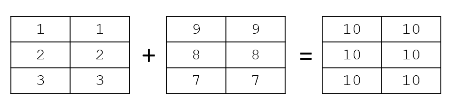
Addition and subtaction across Numpy Arrays are always performed on an element-wise basis. This means that every element in the first array requires a corresponding element in the second array to perform the addition or subtraction operation. Alternatively the calculation must be suitably defined to allow broadcasting of one of the arrays to a common shape.

Addition

Element-wise addition is performed between two arrays using the numpy.add function. You can pass as many arrays to be added as you want to the add function.

NumPy also provides an equivalent shorthand for element-wise addition which is simply the + sign. 

# matrix addition
>>> a = np.array([[1,1],[2,2],[3,3]])
>>> b = np.array([[9,9],[8,8],[7,7]])

>>> c1 = np.add(a,b)
>>> print(c1)
[[10 10]
 [10 10]
 [10 10]]
>>> c2 = a+b+c1 # + is shorthand for .add()
>>> print(c2)
[[20 20]
 [20 20]
 [20 20]]

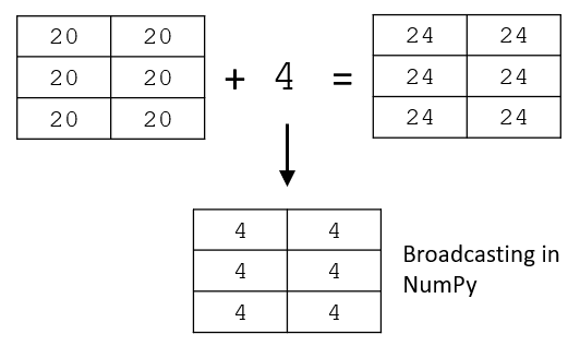
The add function is smart enough to recognise if you are trying to add a scalar value to every element in the array, and will let you do so thanks to broadcasting. 

>>> c3 = c2 + 4 # here we are adding a scaler to an array
>>> print(c3)
[[24 24]
 [24 24]
 [24 24]]

Subraction

Element-wise subtraction in NumPy is performed in exactly the same manner as addition, but making use of the numpy.subtract function. The shorthand for element-wise subtraction is simply the - operator.

>>> a = np.array([[1,1],[2,2],[3,3]])
>>> b = np.array([[9,9],[8,8],[7,7]])

>>> d = np.subtract(b,a)
[[8 8]
 [6 6]
 [4 4]]

>>> d2 = b - a # shorthand for np.subtract()
[[8 8]
 [6 6]
 [4 4]]

Sum

NumPy provides the numpy.sum function which sums all elements along a particular axis.

numpy.sum(a, axis=None, dtype=None, out=None, keepdims=<no value>, initial=<no value>, where=<no value>)

The only required parameter to sum is the array a to be summed. The axis parameter determines along which axis the summation will be completed. The default is None which will sum all the elements in the array and return a single scalar value. You can sum rows or columns in a 2D array by specifying axis=1 or axis=0 respectively. To sum along the last axis in the array set axis=-1.

Flatten Array and Sum

Setting axis=None when applying the sum function will sum all elements in the array and return a single scalar value.

>>> c = np.array([[1,2,3],[4,5,6],[7,8,9]])
>>> print(c)
[[1 2 3]
 [4 5 6]
 [7 8 9]]
>>> sum_c = np.sum(c) # default axis=None 
>>> print(sum_c)
45 # result is a scalar (array flattened)

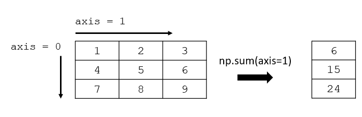
Sum Elements in Row

Elements are summed along each row in a 2D array (matrix) by setting axis=1.

>>> c = np.array([[1,2,3],[4,5,6],[7,8,9]])
>>> sumrows = np.sum(c,axis=1)
>>> print(sumrows)
[ 6 15 24]
>>> print(sumrows.shape)
(3,)

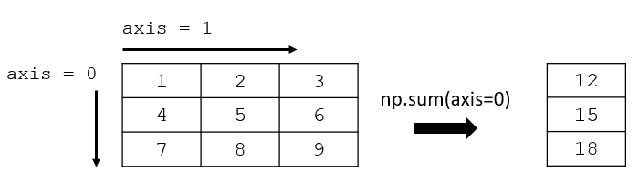
Sum Elements in Column

Elements are summed down each column in a 2D array by setting axis=0 in the sum function.

>>> c = np.array([[1,2,3],[4,5,6],[7,8,9]])
>>> sumcols = np.sum(c,axis=0)
>>> print(sumcols)
[12 15 18]
>>> print(sumcols.shape)
(3,)

Min and Max

Minimum and maximum values in an array can be efficiently determined using the numpy.min and numpy.max functions. As with the sum function, setting the axis parameter determines whether the minimum/maximum of the whole array is output, or a set of minimum/maximum values across thespecified axis.

>>> arr1 = np.arange(16).reshape(4,4)
>>> print(arr1)
[[ 0  1  2  3]
 [ 4  5  6  7]
 [ 8  9 10 11]
 [12 13 14 15]]
>>> print(f"The maximum value is: {arr1.max()}.")
15
>>> print(f"The minimum value is: {arr1.min()}.")
0
# now try find the minimum in each row
>>> minrow = arr1.min(axis=1)
>>> print(minrow)
[ 0  4  8 12]
# now the maximum in each column
>>> maxcol = arr1.max(axis=0)
>>> print(maxcol)
[12 13 14 15]

Broadcasting

We briefly touched on broadcasting when discussing the add and subtract functions but let's now go through it in more detail before turning our attention to the multiplication and division operator.

Broadcasting is the term used by NumPy to describe how arrays with different shapes are treated during arithmetic operations. In cases where broadcasting is possible, the smaller array is broadcast across the larger array in such a way that the arrays have compatible shapes. Remember that arithmetic operations in NumPy are always performed element-wise such that every array in the operation has a correponding element. This allows the operation to be vectorized so that the looping occurs in C and not in Python. This makes the execution much faster, especially when operating on large arrays.

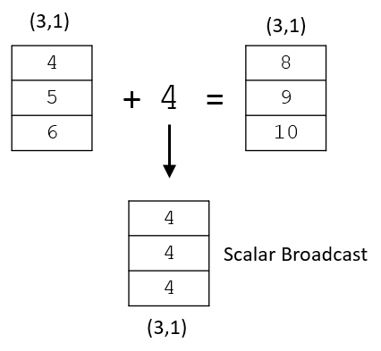
The simplest example of broadcasting to illustrate is an arithmetic operation performed between an array and a scalar. In order for an element-wise calculation to be completed, the scalar value is stretched during the operation into an array with the same shape as the array the scalar is being operated on.

Broadcasting occurs as necessary when performing addition, subtraction, multiplication, and division. It doesn't only apply to operations involving a scalar. In the example below a 1 x 3 array is added to a 3 x 3 array by broadcasting the 1 x 3 to a 3 x 3.

# example of array broadcasting
>>> a = np.array([[1,3,5],[7,8,4],[8,6,2]])
>>> b = np.array([5,8,0])
>>> print(a+b)
[[ 6 11  5]
 [12 16  4]
 [13 14  2]]

If broadcasting is not possible then a ValueError is raised, indicating that the shapes of the arrays are incompatible.

# example of incompatible arithmetic operation and broadcasting failure
>>> a = np.array([[1,3,5],[7,8,4],[8,6,2]])
>>> b = np.array([[5,8,0],[1,2,3]])
>>> print(a+b)
---------------------------------------------------------------------------
ValueError                                Traceback (most recent call last)
~\AppData\Local\Temp\ipykernel_14028\3480802708.py in <module>
      4 b = np.array([[5,8,0],[1,2,3]])
      5 
----> 6 print(a+b)

ValueError: operands could not be broadcast together with shapes (3,3) (2,3)

Multiplication and Division

Multiplication and division follow the broadcasting rules described above.

Arithmetic Multiplication

Multiplication is performed using the np.multiply method, or more commonly with the equivalent operator *. Multiplication is performed element-wise in terms of the broadcasting methods described above.

# Multiplication of a vector by a scalar
>>> matrix1 = np.array([[1,3],[5,7]])
>>> scalar = 5
>>> mult1 = matrix1*scalar
>>> print(mult1)
[[ 5 15]
 [25 35]]

# multiplication of two arrays of equal shape
mat1 = np.array([[6,7],[8,9]])
mat2 = np.array([[5,10],[2,4]])
mat3 = np.multiply(mat1,mat2)
print(mat3)
[[30 70]
 [16 36]]

Arithmetic Division

Division is performed using the np.divide method, or more commonly the equivalent operator /. Multiplication is performed element-wise in terms of the broadcasting described above.

# division by a scalar
>>> todivide = np.array([[5,15],[25,35]])
>>> scalar = 5
>>> div1 = todivide/scalar
>>> print(div1)
[[1. 3.]
 [5. 7.]]

A final example is given below, showing how broadcasting works when dividing two arrays of a different shape.

# division of two arrays
>>> mat4 = np.array([[15,100],[20,40]])
>>> mat5 = np.array([10,2])
>>> mat6 = np.divide(mat4,mat5)
>>> print(mat6)
[[ 1.5 50. ]
 [ 2.  20. ]]

Rounding Operations

We'll finish this tutorial off by looking at a few different rounding type operations that can be completed using the NumPy package. Again the advantage of performing these operations in an ndarray object is that you don't need to write code to loop through the arrays as this is done in the backround using a C routine.

Round

Rounding is performed using the numpy.round function (functionally equivalent to numpy.around). 

numpy.round_(a, decimals=0, out=None)

Specify the number of decimal places to round off to when using the function. The default is to round to the nearest whole number.

>>> pi = np.pi
>>> piarr = np.array([pi,2*pi,3*pi/2,pi/2])
>>> print(piarr)
[3.14159265 6.28318531 4.71238898 1.57079633]

>>> print(np.round(piarr,2))
[3.14 6.28 4.71 1.57]

Floor and Ceiling

Floor and ceiling are common functions that used to ensure conservative results when performing engineering calculations (among many other use cases). The two functions are named numpy.floor and numpy.ceil respectively.

Floor

The floor of scalar x is the largest integer i, such that i <= x.

>>> piarr = np.array([pi,2*pi,3*pi/2,pi/2])
>>> print(piarr)
[3.14159265 6.28318531 4.71238898 1.57079633]
>>> print(np.floor(piarr))
[3. 6. 4. 1.]

Ceiling

The ceil of the scalar x is the smallest integer i, such that i >=x.

>>> piarr = np.array([pi,2*pi,3*pi/2,pi/2])
>>> print(piarr)
[3.14159265 6.28318531 4.71238898 1.57079633]
>>> print(np.ceil(piarr))
[4. 7. 5. 2.]

Truncation

The truncated value of the scalar x is the nearest integer i which is closer to zero than x is. In other words, the fractional part of the number x is discarded in the truncation.

>>> piarr = np.array([pi,2*pi,3*pi/2,pi/2])
>>> print(piarr)
[3.14159265 6.28318531 4.71238898 1.57079633]
>>> print(np.trunc(piarr))
[3. 6. 4. 1.]

Wrapping Up

This concludes our tutorial on basic mathematical functions in NumPy. It's important to remember that the operations covered here are performed element-wise, and where the shapes of the arrays being operated upon are different, then the broadcasting rules apply.

We covered the following topics:

• Looked at the numpy.add and numpy.subtract function. The shorthand for these two operations are + and - respectively.
• We went over the numpy.sum function and showed how summations of arrays can be performed over all elements in the array (flattened) or across any of the array's axes.
• We showed examples of the numpy.min and numpy.max functions.
• Broadcasting was examined, and the concept explained in the context of arithmetic operations.
• Arithmetic multiplication and division of arrays were discussed using the numpy.multiply and numpy.divide functions. The shorthand for these two functions are * and / respectively. 
• Finally we covered the various rounding functions built into NumPy. We specifically touched on numpy.round, numpy.floor, numpy.ceil, and numpy.trunc.

Thanks for reading! If you found this tutorial valuable then please consider sharing it to help us to grow our Python community.